Improving Your SQL Indexing: How to Effectively Order Columns

June 17, 2024

Users often find it hard to choose the best index for a query, especially figuring out the right order of columns.

Imagine you have a large table and you need to filter it to get a specific set of data, which is still quite large. You can use simple conditions like equality or a single range to filter, but your WHERE clause might also include complex conditions with multiple values (IN) and combinations (OR).

After filtering, you only want to show a few rows, ordered by some columns, and limit the results using LIMIT or FETCH FIRST ROWS, typical of pagination. Although indexes help find value ranges and sort results, it’s difficult to decide the best column order for the index when dealing with all these conditions.

Let’s represent this as an SQL statement:

SELECT col4, col5, col3, col6
   FROM large_table
   WHERE col1 = :a
     AND col2 between :b and :c
     AND col3 IN ( 1, 3, 5 ) 
ORDER BY col4 ASC, col5 DESC
LIMIT 10;

This article is divided into two parts. The first part, “How to Find the Best Index,” explains a method that is applicable to all SQL databases. The second part, “A Complete Example,” walks us through the process of optimizing a PostgreSQL query on YugabyteDB and measuring the results using EXPLAIN ANALYZE.

How to Find the Best Index

You should create an efficient index for each table that your query accesses, except for tables from which you need most of the rows, like lookup tables where you hit all keys.

The order of the columns in the key of each index is crucial. It ensures you retrieve only the necessary data, sorted as required, in one or multiple ranges from the index entries stored in the index, which are ordered based on this key.

Column Ordering

When creating a multi-column index, the columns should follow this order from left to right:

The first columns should be for selective equality predicates, and they can be HASH in YugabyteDB when there’s millions of values to distribute.
An example in the query is: WHERE col1 = :a
Next, include columns used with a range predicates that results in a single range, such as an inequality, and they can be defined as ASC or DESC
An example in the query is: WHERE col2 between :b and :c
If you want to avoid a sort, which is essential for pagination queries, include the columns to order on using the same ASC and DESC as in your ORDER BY
An example in the query is: ORDER BY col4 ASC, col5 DESC
Finally, include the columns for other selective predicates, which would lead to multiple ranges if placed before the ordering columns, and then wouldn’t provide one globally ordered result. They can be in INCLUDE or at the end of the key
An example in the query is: WHERE col3 IN ( 1, 3, 5 )
You can include all other columns to get all the results from the index
An example in the query is: SELECT col4, col5, col3, col6

It’s important to consider trade-offs. For instance, you might have very selective multi-value criteria and decide to swap steps 3 and 4, to benefit from skip scan reading multiple ranges. However, this comes at the price of adding a sort operation during execution. Looking at the execution plan and execution statistics helps you to understand the difference, which I’ll show later in the example.

Index Scan Ranges

When using indexes to return rows in a specific order, it’s crucial to understand the difference between a single range and multiple ranges. Essentially, you can think of any index as being sorted based on the concatenation of the columns of its key.

Some predicates allow you to seek to one key and read from there in order. YugabyteDB can seek to multiple ranges when you have a list of values for an IN predicate. It preserves the order of rows from the preceding columns. However, the columns after it will only be ordered within each range.

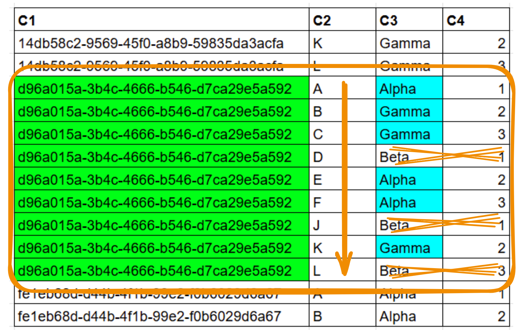
Let’s take the following example:

SELECT * from table 
 WHERE C1 = 'd96a015a-3b4c-4666-b546-d7ca29e5a592' 
   AND C3 in ('Alpha','Gamma')
 ORDER BY C2

An index on ( C1, C2, C3, C4 ) will scan a single range of 9 rows. It will have to discard 3 rows later, but gets the result ordered without additional sort:

single range index scan preserving the order but reading more entries

An index on ( C1, C3, C2, C4 ) will scan scan two smaller ranges with no need for an additional filter, however it requires a sort operation because it is only partially ordered:

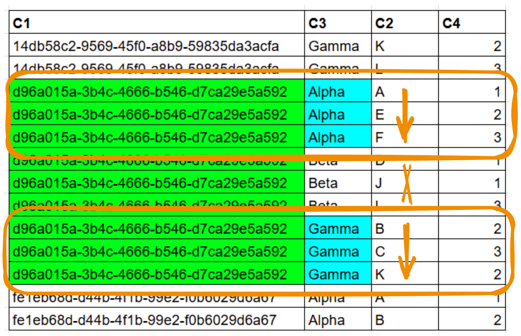
multiple ranges index skip scan to read less entries, but not matching the order by

In this situation, the most efficient index will depend on your data. If the predicate on column C3 is very selective, there’s a large benefit in skipping between multiple ranges rather than scanning one larger range. If the result is small, a sort operation is not a problem. If the scan result returns lot of rows that have to be ordered, like for pagination queries, the benefit of getting rows in order from a single range outweighs that of skipping few rows when reading.

Index Scan Capabilities

This method is applicable to most databases, with some exceptions. The HASH option is for distributed databases that support hash sharding in addition to range sharding (for example, YugabyteDB does, but Spanner, CockroachDB and TiDB do not).

The multiple-range option is for databases that support skip scan (for example, YugabyteDB and Oracle do, but PostgreSQL does not).

The INCLUDE option is for databases that support it (YugabyteDB and PostgreSQL do, but Oracle does not). It is easy to work around by putting the columns at the end of the key.

The partial index option (WHERE) is for databases that support it (YugabyteDB and PostgreSQL do, but Oracle does not) and is more difficult to work around (with partitioning or function-based indexes).

I’ll demonstrate how we can create the best index for a specific query using YugabyteDB, as it provides all the capabilities detailed above. I’ll do this in multiple steps because you do not need to use all capabilities. It is important to evaluate the benefit when creating a new index or adding a column to an existing index. You may create an index that is good enough for your performance criteria, especially if it can serve many other queries.

A Complete Example

To illustrate the method, I’ll go through an example, looking at the execution plan, trying some indexes, and showing the results. I used YugabyteDB 2.21 with the following table:

drop schema if exists demo cascade;

CREATE SCHEMA IF NOT EXISTS demo;
CREATE TABLE demo.events (
    id UUID NOT NULL,
    system_id UUID NOT NULL,
    event_type VARCHAR(100) NOT NULL,
    created_at TIMESTAMPTZ NOT NULL,
    updated_at TIMESTAMPTZ NOT NULL,
    state VARCHAR(100) NOT NULL,
    customer_id UUID,
    device UUID,
    PRIMARY KEY (id)
);
CREATE INDEX events_system_id ON demo.events
 (system_id);

An index has been created on “system_id” because we know that it is a selective criterion in many queries. We will look at one such query. I want to fetch a batch of events pertaining to a particular system, ordered by their creation date. I have some additional filters on type and state and will display only the first hundred rows.

Execution Plan

My query is simple: for one “system_id”, get the events with some “event_type” and “state”. I provide a list of values for those. The result might be large, but I’m interested in the Top-100 when ordered by “created_at” date. Here is the query and its execution plan:

yugabyte=# EXPLAIN (costs off)
SELECT *
FROM demo.events
WHERE events.system_id = '0188e8d7-dead-73c1-b218-7cf069921b5b'
 AND (
  events.event_type IN (
   'ONBOARDING',
   'MONITORING',
   'TRANSFERRING'
  )
  AND
  events.state IN (
   'EVENT_NOT_STARTED',
   'EVENT_IN_PROGRESS',
   'EVENT_MONITORING_NOT_STARTED'
  )
)
ORDER BY events.created_at ASC LIMIT 100;
                                                                                                                                                          QUERY PLAN
-------------------------------------------------------------------------------
 Limit
   ->  Sort
         Sort Key: created_at
         ->  Index Scan using events_system_id on events
               Index Cond: (system_id = '0188e8d7-dead-73c1-b218-7cf069921b5b'::uuid)
               Filter: (((event_type)::text = ANY ('{ONBOARDING,MONITORING,TRANSFERRING}'::text[])) AND ((state)::text = ANY ('{EVENT_NOT_STARTED,EVENT_IN_PROGRESS,EVENT_MONITORING_NOT_STARTED}'::text[])))

If you are used to reading execution plans, you already know the problem we need to solve. We have a good index for our most selective filter, the “system_id” being in the Index Condition. However, the most selective filtering, the LIMIT, occurs after the Sort operation, and a Sort operation has to read all rows and sort them before being able to return the first ones.

In short, the response time will be proportional to the number of events for one “system_id,” but not to the result fetched by the user. This will not scale.

Testing With Data

When we have data in the table, we can run the query with EXPLAIN ANALYZE showing the number of rows. I’m inserting one million rows here (using non-transactional writes to make the bulk load faster as nobody queries it):

CREATE EXTENSION IF NOT EXISTS pgcrypto;

--- Use non-transactional writes for fast bulk load in YugabyteDB
set yb_disable_transactional_writes=on;

INSERT INTO demo.events (id, system_id, event_type, created_at, updated_at, state, customer_id, device)
SELECT
    gen_random_uuid(), -- id
    case when random()>0.8 then '0188e8d7-dead-73c1-b218-7cf069921b5b' else gen_random_uuid() end, -- system_id
    (ARRAY['ONBOARDING', 'MONITORING', 'TRANSFERRING', 'MAINTENANCE', 'UPGRADE'])[floor(random() * 5 + 1)], -- event_type
    NOW() - interval '1 year' * random(), -- created_at (random time within the last year)
    NOW() - interval '1 year' * random(), -- updated_at (random time within the last year)
    (ARRAY['EVENT_NOT_STARTED', 'EVENT_IN_PROGRESS', 'EVENT_MONITORING_NOT_STARTED', 'EVENT_MONITORING_IN_PROGRESS', 'EVENT_PAYMENT_SCREENING_NOT_STARTED', 'EVENT_PAYMENT_SCREENING_IN_PROGRESS', 'EVENT_TRANSFERRING_NOT_STARTED', 'EVENT_TRANSFERRING_IN_PROGRESS', 'EVENT_COMPLETED', 'EVENT_CANCELLED'])[floor(random() * 10 + 1)], -- state
    gen_random_uuid(), -- customer_id
    gen_random_uuid() -- device
FROM generate_series(1, 1000000);

--- Reset the transactional writes to be fully ACID
set yb_disable_transactional_writes=off;

The advantage of having data is being able to look at the execution statistics in terms of read requests and number of rows scanned and fetched. I don’t care about the total response time because it depends on many parameters, like the cache hits, which are different from production when I’m testing. My first run in a test environment starts with a cold cache, the next runs have an irrealistic cache hit ratio.

Explain Analyze

The most important metric to understand the actual cost of an execution plan, is the number of buffer reads by PostgreSQL, or the number of distributed read requests on YugabyteDB, respectively gathered with EXPLAIN (ANALYZE, BUFFERS) and EXPLAIN (ANALYZE, DIST).

My query takes one second to return a hundred rows. From a user point of view, this is difficult to understand, but with EXPLAIN ANALYZE, this time can be explained by the number of PostgreSQL Buffers or YugabyteDB Read Requests. I run it with YugabyteDB, which additionally shows the number of rows scanned from the index and the table so that we can understand exactly what happens:

yugabyte=# EXPLAIN (analyze, dist, verbose, costs off)
SELECT *
FROM demo.events
WHERE events.system_id = '0188e8d7-dead-73c1-b218-7cf069921b5b'
 AND (
  events.event_type IN (
   'ONBOARDING',
   'MONITORING',
   'TRANSFERRING'
  )
  AND
  events.state IN (
   'EVENT_NOT_STARTED',
   'EVENT_IN_PROGRESS',
   'EVENT_MONITORING_NOT_STARTED'
  )
)
ORDER BY events.created_at ASC LIMIT 100;
                                                                                                                                                                    QUERY PLAN
-------------------------------------------------------------------------------        Limit (actual time=1100.385..1100.428 rows=100 loops=1)
   Output: id, system_id, event_type, created_at, updated_at, state, customer_id, device
   ->  Sort (actual time=1100.383..1100.398 rows=100 loops=1)
         Output: id, system_id, event_type, created_at, updated_at, state, customer_id, device
         Sort Key: events.created_at
         Sort Method: top-N heapsort  Memory: 71kB
         ->  Index Scan using events_system_id on demo.events (actual time=8.067..1084.709 rows=35989 loops=1)
               Output: id, system_id, event_type, created_at, updated_at, state, customer_id, device
               Index Cond: (events.system_id = '0188e8d7-dead-73c1-b218-7cf069921b5b'::uuid)
               Filter: (((events.event_type)::text = ANY ('{ONBOARDING,MONITORING,TRANSFERRING}'::text[])) AND ((events.state)::text = ANY ('{EVENT_NOT_STARTED,EVENT_IN_PROGRESS,EVENT_MONITORING_NOT_STARTED}'::text[])))
               Rows Removed by Filter: 164551
               Storage Table Read Requests: 196
               Storage Table Read Execution Time: 872.751 ms
               Storage Table Rows Scanned: 200540
               Storage Index Read Requests: 196
               Storage Index Read Execution Time: 2.413 ms
               Storage Index Rows Scanned: 200540
 Planning Time: 0.119 ms
 Execution Time: 1100.717 ms

To return those hundred rows, we have read two hundred thousand index entries from the secondary index, and the same amount of rows from the table.

If we look at the timings, reading from the table was much more expensive (800 milliseconds) than reading from the index (2 milliseconds). The reason for this is that we read a single range from the index, which starts with the index condition column, but the rows are scattered in the table, in the order where they arrived in PostgreSQL heap tables, or in the order of their primary key for YugabyteDB LSM Tree.

Let’s address this point first, which is visible as ‘Rows Removed by Filter’. There are 164551 rows that are read and then discarded to get 35989 rows from the Index Scan operation. Can we discard them before going to the table? My optimization goal is to get no rows removed by filter, like this:

Rows Removed by Filter: 0
Storage Table Rows Scanned: 35989
Storage Index Rows Scanned: 35989

Read Less Rows From the Table

If the index has the value of “event_type” and “state” added to the index entry, the filter can be applied before going to the table. I can add them at the end of the index key or as additional INCLUDE’d columns. Here are the possible indexes I can create to achieve this goal:

create index i1_ies  on demo.events (system_id, event_type, state);
create index i1_ie_s on demo.events (system_id, event_type) include (state);
create index i1_i_es on demo.events (system_id) include (event_type, state);

create index i1_ise  on demo.events (system_id, state, event_type);
create index i1_is_e on demo.events (system_id, state) include (event_type);
create index i1_i_se on demo.events (system_id) include (state, event_type);

create index i1_i_se on demo.events (system_id) include (state, event_type);

All those indexes achieve the same goals for this query. The choice depends on other queries and that’s why you should have a good overview of your access patterns.

If the columns are frequently updated, it may be more efficient to have them in INCLUDE (and here the order of columns do not matter) rather than in the key. But, most important, you want indexes that are used for multiple queries to avoid creating too many of them. Adding a column to the key may help another query with a selective predicate, or ordering on it, after filtering on the previous key columns.

Here I choose to put all in the key, with the “state” first, because I may have queries on one “system_id” and one “state” with low cardinality:

-- access by single "system_id" and multi-value filter on "state" and "event_type" by query XYZ
create index i1_ise  on demo.events (system_id, state, event_type);

Note: it is a good idea to document the choice of the index so that when you are tuning another query you know what you can change in the index, and what must be there. That’s why I’ve put a comment.

With this index, I run my EXPLAIN ANALYZE again

yugabyte=# EXPLAIN (analyze, dist, verbose, costs off)
SELECT *
FROM demo.events
WHERE events.system_id = '0188e8d7-dead-73c1-b218-7cf069921b5b'
 AND (
  events.event_type IN (
   'ONBOARDING',
   'MONITORING',
   'TRANSFERRING'
  )
  AND
  events.state IN (
   'EVENT_NOT_STARTED',
   'EVENT_IN_PROGRESS',
   'EVENT_MONITORING_NOT_STARTED'
  )
)
ORDER BY events.created_at ASC LIMIT 100;
                                                                                                                                                   QUERY PLAN
------------------------------------------------------------------------------- Limit (actual time=285.903..285.946 rows=100 loops=1)
   Output: id, system_id, event_type, created_at, updated_at, state, customer_id, device
   ->  Sort (actual time=285.735..285.750 rows=100 loops=1)
         Output: id, system_id, event_type, created_at, updated_at, state, customer_id, device
         Sort Key: events.created_at
         Sort Method: top-N heapsort  Memory: 69kB
         ->  Index Scan using i1_ise on demo.events (actual time=16.487..273.870 rows=35989 loops=1)
               Output: id, system_id, event_type, created_at, updated_at, state, customer_id, device
               Index Cond: ((events.system_id = '0188e8d7-dead-73c1-b218-7cf069921b5b'::uuid) AND ((events.state)::text = ANY ('{EVENT_NOT_STARTED,EVENT_IN_PROGRESS,EVENT_MONITORING_NOT_STARTED}'::text[])) AND ((events.event_type)::text = ANY ('{ONBOARDING,MONITORING,TRANSFERRING}'::text[])))
               Storage Table Read Requests: 36
               Storage Table Read Execution Time: 214.989 ms
               Storage Table Rows Scanned: 35989
               Storage Index Read Requests: 36
               Storage Index Read Execution Time: 2.894 ms
               Storage Index Rows Scanned: 35989
 Planning Time: 18.095 ms
 Execution Time: 287.947 ms

My goal is achieved: no more Rows Removed By Filter.

The filtering happens when reading the index entries. This is good, but we can do better. At the end, we return 100 rows, so ideally, we should scan no more than those 100 rows. My new tuning goal is:

Rows Removed by Filter: 0
Storage Table Rows Scanned: 100
Storage Index Rows Scanned: 100

Index Condition: Access, Skip Scan, and Filter

Before looking at this optimization goal, I can reduce the time it takes to read 163539 index entries and filter them down to 36055.

It is not visible in the PostgreSQL execution plan, but the Index Condition has two categories of predicates.

One: the access condition, used to seek into the index to read a range, skipping the rows that do not verify the condition
Two: the filtering that is applied after reading the rows.

In my example, “system_id” is an access filter, and “state” and “event_type” are filters.

With YugabyteDB, there’s an additional optimization where one access filter can read multiple ranges, often called Skip Scan or Loose Index Scan. This may influence the decision to put columns at the end of the key or in INCLUDE.

Let’s forget about the ORDER BY for now. In addition to the DIST option of EXPLAIN ANALYZE, I use the DEBUG option that shows all details about the reads: the number of times we skip to a range in the index, visible as RocksDB ‘seek’, and the number of times we read the next row within the range, visible as RocksDB ‘next’.

With a predicate on “system_id” only:

yugabyte=# EXPLAIN (analyze, dist, debug, verbose, costs off, summary off)
select count(*) from demo.events
WHERE events.system_id = '0188e8d7-dead-73c1-b218-7cf069921b5b';
 

QUERY PLAN
------------------------------------------------------------------------------- 
 Finalize Aggregate (actual time=96.487..96.487 rows=1 loops=1)
   Output: count(*)
   ->  Index Only Scan using events_system_id on demo.events (actual time=96.471..96.474 rows=1 loops=1)
         Index Cond: (events.system_id = '0188e8d7-dead-73c1-b218-7cf069921b5b'::uuid)
         Heap Fetches: 0
         Storage Index Read Requests: 1
         Storage Index Read Execution Time: 96.121 ms
         Storage Index Rows Scanned: 200540
         Metric rocksdb_number_db_seek: 1.000
         Metric rocksdb_number_db_next: 200540.000
         Metric rocksdb_number_db_seek_found: 1.000
         Metric rocksdb_number_db_next_found: 200540.000
         Metric rocksdb_iter_bytes_read: 15180876.000
         Metric docdb_keys_found: 200540.000
         Metric ql_read_latency: sum: 94551.000, count: 1.000
         Partial Aggregate: true

Because “system_id” is the first column of the index, I have to read a single range. This is visible with 1 “seek” into the LSM tree key. I read all rows within this range: 200540 “next” key-values are read.

If I add the predicates on “event_type” and “state”, rather than reading one range and filtering afterwards, I can read multiple smaller ranges:

yugabyte=# EXPLAIN (analyze, dist, debug, verbose, costs off, summary off)
select count(*) from demo.events
WHERE events.system_id = '0188e8d7-dead-73c1-b218-7cf069921b5b'
 AND (
  events.event_type IN (
   'ONBOARDING',
   'MONITORING',
   'TRANSFERRING'
  )
  AND
  events.state IN (
   'EVENT_NOT_STARTED',
   'EVENT_IN_PROGRESS',
   'EVENT_MONITORING_NOT_STARTED'
  )
)
;

QUERY PLAN
------------------------------------------------------------------------------- 
 Finalize Aggregate (actual time=29.118..29.119 rows=1 loops=1)
   Output: count(*)
   ->  Index Only Scan using i1_ise on demo.events (actual time=28.931..28.935 rows=1 loops=1)
         Index Cond: ((events.system_id = '0188e8d7-dead-73c1-b218-7cf069921b5b'::uuid) AND (events.state = ANY ('{EVENT_NOT_STARTED,EVENT_IN_PROGRESS,EVENT_MONITORING_NOT_STARTED}'::text[])) AND (events.event_type = ANY ('{ONBOARDING,MONITORING,TRANSFERRING}'::text[])))
         Heap Fetches: 0
         Storage Index Read Requests: 1
         Storage Index Read Execution Time: 26.137 ms
         Storage Index Rows Scanned: 35989
         Metric rocksdb_number_db_seek: 3.000
         Metric rocksdb_number_db_next: 35993.000
         Metric rocksdb_number_db_seek_found: 3.000
         Metric rocksdb_number_db_next_found: 35993.000
         Metric rocksdb_iter_bytes_read: 4060397.000
         Metric docdb_keys_found: 35989.000
         Metric ql_read_latency: sum: 23425.000, count: 1.000
         Partial Aggregate: true

Here, instead of reading 200540 rows from one range, and filtering on “state” and “event_type” later, it has read 3 ranges and a total of 35993 because it has skipped the values that were not in the IN clause. YugabyteDB builds a combination of the possible ranges to minimize the read requests.

To understand it better, the best way is to visualize the order of the index. To show it, I query the table with an ORDER BY that matches the index key. I also GROUP BY just to make the display smaller, and I add a CASE statement to show which rows verify the WHERE clause. Here is my query that visualizes my index content:

select
 case when
 events.system_id = '0188e8d7-dead-73c1-b218-7cf069921b5b'
 AND (
  events.event_type IN (
   'ONBOARDING',
   'MONITORING',
   'TRANSFERRING'
  )
  AND
  events.state IN (
   'EVENT_NOT_STARTED',
   'EVENT_IN_PROGRESS',
   'EVENT_MONITORING_NOT_STARTED'
  )
) then '✅' else '❌' end keep
,     system_id, state, event_type
,count(*)
from demo.events
where system_id = '0188e8d7-dead-73c1-b218-7cf069921b5b'
GROUP BY system_id, state, event_type
ORDER BY system_id, state, event_type
;

and here is the output:

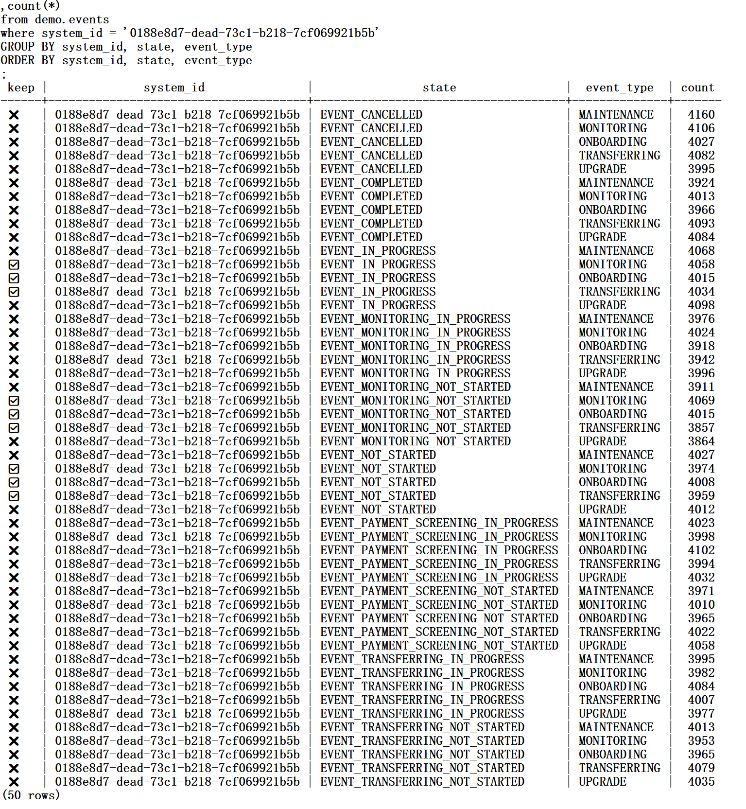
screenshot showing rows ordered like in the index, and three ranges that verify the WHERE clause

This method makes it easy to understand the 3 seeks and 35993 next:

one to go to | 0188e8d7-dead-73c1-b218-7cf069921b5b | EVENT_IN_PROGRESS | MONITORING | , reading 4058 + 4015 + 4034 = 12107 index entries
one to go to | 0188e8d7-dead-73c1-b218-7cf069921b5b | EVENT_MONITORING_NOT_STARTED | MONITORING |, reading 4069 + 4015 + 3857 = 11941 index entries
one to go to | 0188e8d7-dead-73c1-b218-7cf069921b5b | EVENT_NOT_STARTED | MONITORING | , reading 3974 + 4008 + 3959 = 11941 index entries

There’s no magic. The number of ‘seek’ and ‘next’ comes directly from the physical order of the index and the ranges that verify the WHERE clause.

The best access path is to get all rows with one or a few ranges without reading too much that is not needed for the result. The art of indexing is to provide a structure that stores index entries in this order.

Partial Index

If the list of values is fairly static, all queries using the same, we can skip them even earlier, before the execution, at planning time. With partial indexes, we can create an index that stores only the entries that validate a where clause.

create index i1_i_partial  on demo.events (system_id) 
where (
  events.event_type IN (
   'ONBOARDING',
   'MONITORING',
   'TRANSFERRING'
  )
  AND
  events.state IN (
   'EVENT_NOT_STARTED',
   'EVENT_IN_PROGRESS',
   'EVENT_MONITORING_NOT_STARTED'
  )
);

With this index, I run my COUNT(*) query from above to see that the three “seek” has been reduced to only one:

EXPLAIN (analyze, dist, debug, verbose, costs off, summary off)
select count(*) from demo.events
WHERE events.system_id = '0188e8d7-dead-73c1-b218-7cf069921b5b'
 AND (
  events.event_type IN (
   'ONBOARDING',
   'MONITORING',
   'TRANSFERRING'
  )
  AND
  events.state IN (
   'EVENT_NOT_STARTED',
   'EVENT_IN_PROGRESS',
   'EVENT_MONITORING_NOT_STARTED'
  )
)
;
                                             QUERY PLAN
-------------------------------------------------------------------------------
 Finalize Aggregate (actual time=11.943..11.943 rows=1 loops=1)
   Output: count(*)
   ->  Index Only Scan using i1_i_partial on demo.events (actual time=11.930..11.933 rows=1 loops=1)
         Index Cond: (events.system_id = '0188e8d7-dead-73c1-b218-7cf069921b5b'::uuid)
         Heap Fetches: 0
         Storage Index Read Requests: 1
         Storage Index Read Execution Time: 11.710 ms
         Storage Index Rows Scanned: 35989
         Metric rocksdb_number_db_seek: 1.000
         Metric rocksdb_number_db_next: 35989.000
         Metric rocksdb_number_db_seek_found: 1.000
         Metric rocksdb_number_db_next_found: 35989.000
         Metric rocksdb_iter_bytes_read: 2702969.000
         Metric docdb_keys_found: 35989.000
         Metric ql_read_latency: sum: 10997.000, count: 1.000
         Partial Aggregate: true

You can see that the conditions on “state” and “event_type” are not even visible in the execution plan, because the partial index guarantees that all index entries validate this condition.

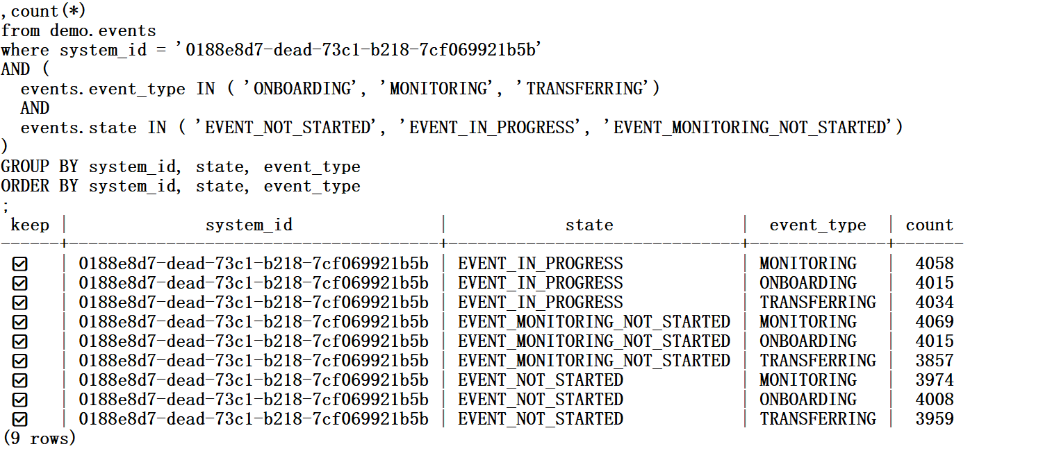
The partial index has only one range that validates my condition, like this:

screenshot showing rows ordered like in the index, with only one range that satisfies the WHERE clause

Back to my main query, with this partial index, to see how it benefits from it:

yugabyte=# EXPLAIN (analyze, dist, verbose, costs off)
SELECT *
FROM demo.events
WHERE events.system_id = '0188e8d7-dead-73c1-b218-7cf069921b5b'
 AND (
  events.event_type IN (
   'ONBOARDING',
   'MONITORING',
   'TRANSFERRING'
  )
  AND
  events.state IN (
   'EVENT_NOT_STARTED',
   'EVENT_IN_PROGRESS',
   'EVENT_MONITORING_NOT_STARTED'
  )
)
ORDER BY events.created_at ASC LIMIT 100;
                                                QUERY PLAN
-------------------------------------------------------------------------------  Limit (actual time=239.850..239.893 rows=100 loops=1)
   Output: id, system_id, event_type, created_at, updated_at, state, customer_id, device
   ->  Sort (actual time=239.849..239.863 rows=100 loops=1)
         Output: id, system_id, event_type, created_at, updated_at, state, customer_id, device
         Sort Key: events.created_at
         Sort Method: top-N heapsort  Memory: 71kB
         ->  Index Scan using i1_i_partial on demo.events (actual time=8.853..227.843 rows=35989 loops=1)
               Output: id, system_id, event_type, created_at, updated_at, state, customer_id, device
               Index Cond: (events.system_id = '0188e8d7-dead-73c1-b218-7cf069921b5b'::uuid)
               Storage Table Read Requests: 36
               Storage Table Read Execution Time: 192.771 ms
               Storage Table Rows Scanned: 35989
               Storage Index Read Requests: 36
               Storage Index Read Execution Time: 2.210 ms
               Storage Index Rows Scanned: 35989
 Planning Time: 0.431 ms
 Execution Time: 240.145 ms

Execution is a bit faster because the index is smaller. Partial indexes are also lighter to maintain because inserts that have other values do not have an entry to add. However, you should evaluate the benefits of it.

If the non-partial index is still needed for other queries, then it is better to maintain one index that is good enough for both queries, rather than adding an index that saves a few milliseconds. In my case, I have no queries that need this access by “system_id” for other “state” or “event_type” so I can remove the non-partial one.

yugabyte=# drop index demo.i1_ise ;
DROP INDEX

Fetch Size

I have seen that the 35989 rows I’m reading fit in only one range, but if you run the query with the DEBUG option you will see 36 ‘seek’. The reason is that by default the rows are fetched by 1024, so that 36055 is fetched with 36 read requests and each one will seek to the next place with a new iterator. We will see later how to reduce the number of rows, which is the best approach, but if you cannot, you can reduce the number of fetches. The default fetch size is 1024:

yugabyte=# \dconfig yb_fetch*
List of configuration parameters
      Parameter      | Value
---------------------+-------
 yb_fetch_row_limit  | 1024
 yb_fetch_size_limit | 0
(2 rows)

Here is my query after increasing the fetch size to 100000 to reduce the number of read requests to its minimum (but you must be aware that it increases the memory footprint).

yugabyte=# set yb_fetch_row_limit = 100000;
SET

yugabyte=# EXPLAIN (analyze, dist, verbose, costs off)
SELECT *
FROM demo.events
WHERE events.system_id = '0188e8d7-dead-73c1-b218-7cf069921b5b'
 AND (
  events.event_type IN (
   'ONBOARDING',
   'MONITORING',
   'TRANSFERRING'
  )
  AND
  events.state IN (
   'EVENT_NOT_STARTED',
   'EVENT_IN_PROGRESS',
   'EVENT_MONITORING_NOT_STARTED'
  )
)
ORDER BY events.created_at ASC LIMIT 100;
                                                 QUERY PLAN
-------------------------------------------------------------------------------
 Limit (actual time=164.904..164.945 rows=100 loops=1)
   Output: id, system_id, event_type, created_at, updated_at, state, customer_id, device
   ->  Sort (actual time=164.902..164.913 rows=100 loops=1)
         Output: id, system_id, event_type, created_at, updated_at, state, customer_id, device
         Sort Key: events.created_at
         Sort Method: top-N heapsort  Memory: 71kB
         ->  Index Scan using i1_i_partial on demo.events (actual time=133.531..153.172 rows=35989 loops=1)
               Output: id, system_id, event_type, created_at, updated_at, state, customer_id, device
               Index Cond: (events.system_id = '0188e8d7-dead-73c1-b218-7cf069921b5b'::uuid)
               Storage Table Read Requests: 1
               Storage Table Read Execution Time: 91.142 ms
               Storage Table Rows Scanned: 35989
               Storage Index Read Requests: 1
               Storage Index Read Execution Time: 19.848 ms
               Storage Index Rows Scanned: 35989
 Planning Time: 4.025 ms
 Execution Time: 165.420 ms

With a larger fetch size, I got all rows with a single read request (and one ‘seek’ if you run it with DEBUG).

But we can do better. If we read only what is needed, 100 rows, we don’t need to increase the fetch size. The problem is that I read 35989 rows, fetched them from the distributed storage, sorted them, and finally kept the Top-100 of them. Indexes store their entries in the order of the key, so it can help to avoid the sort operation.

Order-Preserving Index

I’ll add CREATED_AT in the index. The dilemma is where to place it.

I don’t want to place it before “system_id” because then my index entries for one “system_id” would be scattered in the index, seeking too many ranges.

I don’t want to place them after “state” and “event_type” because I read multiple values for them. If you remember that there are 3 ranges. Having each range in the right order doesn’t help to get the final result in this order. This would necessitate at least a merge sort.

The best solution is to place “created_at” before the columns that split the range into multiple ones. I create this index:

create index i1_icse 
 on demo.events (system_id, created_at, state, event_type);

This will not benefit from skip scan on “state” and “event_type,” but it gets the rows in order and then filters them, preserving the order. It not only avoids the cost of sorting, but also avoids reading all rows.

It may depends on the data distribution and selectivity, but in my case avoiding having to read and sort a large row set has a much greater benefit than filtering faster on “state” and “event_type”.

Without the cost-based optimizer, the index is not picked up (the rules do not consider the cost of the Sort and Limit operation), but I can use a hint to force it:

yugabyte=# EXPLAIN (analyze, dist, verbose, costs off)
/*+ IndexScan(events i1_icse ) */
SELECT *
FROM demo.events
WHERE events.system_id = '0188e8d7-dead-73c1-b218-7cf069921b5b'
 AND (
  events.event_type IN (
   'ONBOARDING',
   'MONITORING',
   'TRANSFERRING'
  )
  AND
  events.state IN (
   'EVENT_NOT_STARTED',
   'EVENT_IN_PROGRESS',
   'EVENT_MONITORING_NOT_STARTED'
  )
)
ORDER BY events.created_at ASC LIMIT 100;
                                                                                                                                                QUERY PLAN
-------------------------------------------------------------------------------  Limit (actual time=7.066..7.148 rows=100 loops=1)
   Output: id, system_id, event_type, created_at, updated_at, state, customer_id, device
   ->  Index Scan using i1_icse on demo.events (actual time=7.063..7.118 rows=100 loops=1)
         Output: id, system_id, event_type, created_at, updated_at, state, customer_id, device
         Index Cond: ((events.system_id = '0188e8d7-dead-73c1-b218-7cf069921b5b'::uuid) AND ((events.state)::text = ANY ('{EVENT_NOT_STARTED,EVENT_IN_PROGRESS,EVENT_MONITORING_NOT_STARTED}'::text[])) AND ((events.event_type)::text = ANY ('{ONBOARDING,MONITORING,TRANSFERRING}'::text[])))
         Storage Table Read Requests: 1
         Storage Table Read Execution Time: 2.151 ms
         Storage Table Rows Scanned: 100
         Storage Index Read Requests: 1
         Storage Index Read Execution Time: 2.972 ms
         Storage Index Rows Scanned: 100
 Planning Time: 16.009 ms
 Execution Time: 8.685 ms

This is exactly what I wanted to see: it reads only 100 rows from the index.

With the tables analyzed and the Cost Based Optimizer enabled, the right index is chose without the need of a hint:

yugabyte=# analyze demo.events;
ANALYZE

yugabyte=# set yb_enable_base_scans_cost_model=on;
SET

yugabyte=# EXPLAIN
SELECT *
FROM demo.events
WHERE events.system_id = '0188e8d7-dead-73c1-b218-7cf069921b5b'
 AND (
  events.event_type IN (
   'ONBOARDING',
   'MONITORING',
   'TRANSFERRING'
  )
  AND
  events.state IN (
   'EVENT_NOT_STARTED',
   'EVENT_IN_PROGRESS',
   'EVENT_MONITORING_NOT_STARTED'
  )
)
ORDER BY events.created_at ASC LIMIT 100;
                                                                                                                                QUERY PLAN
-------------------------------------------------------------------------------
 Limit  (cost=16.89..12358.54 rows=100 width=116)
   ->  Index Scan using i1_icse on events  (cost=16.89..123416541.94 rows=1000000 width=116)
         Index Cond: ((system_id = '0188e8d7-dead-73c1-b218-7cf069921b5b'::uuid) AND ((state)::text = ANY ('{EVENT_NOT_STARTED,EVENT_IN_PROGRESS,EVENT_MONITORING_NOT_STARTED}'::text[])) AND ((event_type)::text = ANY ('{ONBOARDING,MONITORING,TRANSFERRING}'::text[])))

Here, I displayed the estimated cost. It shows exactly where our optimization comes from: the cost of this index scan is large but limiting to read only 100 rows it is 123416541 / 12358.54 = 10000x less expensive.

In reality, I don’t need the hint because the other indexes are not required. Even with the rule based optimizer, my new index is picked up if I remove the partial index.

yugabyte=# drop index demo.i1_i_partial;
DROP INDEX

With EXPLAIN I check that my index is picked up:

yugabyte=# EXPLAIN (analyze, dist, verbose, costs off)
SELECT *
FROM demo.events
WHERE events.system_id = '0188e8d7-dead-73c1-b218-7cf069921b5b'
 AND (
  events.event_type IN (
   'ONBOARDING',
   'MONITORING',
   'TRANSFERRING'
  )
  AND
  events.state IN (
   'EVENT_NOT_STARTED',
   'EVENT_IN_PROGRESS',
   'EVENT_MONITORING_NOT_STARTED'
  )
)
ORDER BY events.created_at ASC LIMIT 100;
                                                                                                                                                QUERY PLAN
------------------------------------------------------------------------------- Limit (actual time=3.658..3.742 rows=100 loops=1)
   Output: id, system_id, event_type, created_at, updated_at, state, customer_id, device
   ->  Index Scan using i1_icse on demo.events (actual time=3.654..3.711 rows=100 loops=1)
         Output: id, system_id, event_type, created_at, updated_at, state, customer_id, device
         Index Cond: ((events.system_id = '0188e8d7-dead-73c1-b218-7cf069921b5b'::uuid) AND ((events.state)::text = ANY ('{EVENT_NOT_STARTED,EVENT_IN_PROGRESS,EVENT_MONITORING_NOT_STARTED}'::text[])) AND ((events.event_type)::text = ANY ('{ONBOARDING,MONITORING,TRANSFERRING}'::text[])))
         Storage Table Read Requests: 1
         Storage Table Read Execution Time: 1.413 ms
         Storage Table Rows Scanned: 100
         Storage Index Read Requests: 1
         Storage Index Read Execution Time: 1.730 ms
         Storage Index Rows Scanned: 100
 Planning Time: 0.129 ms
 Execution Time: 3.815 ms

With this index, on this dataset, your optimization goal is probably reached, as the total execution time is less than 5 milliseconds. But, if you read more rows, you may want to avoid the read requests to the table rows with a covering index.

The new challenge is:

Rows Removed by Filter: 0
Storage Table Rows Scanned: 0
Storage Index Rows Scanned: 100

Index Only Scan

I already mentioned that adding columns to the index, at the end of the key or in the INCLUDE clause, can optimize the scan by covering the columns used in the where clause.

We have covered the columns used in the ORDER BY to avoid a sort. We can also cover all columns that are selected to aim for an Index Only Scan. If all columns used by the query are in the index entries, in the key or INCLUDE part, there’s no need to read the table. This is often called ‘covering index,’ but keep in mind that one index can cover one query and not another.

Let’s include the columns that are not already in the key:

create index i1_icse_covering  
on demo.events (system_id, created_at, state, event_type) 
include (id, updated_at, customer_id, device);

It is easy to know which columns to add because I’ve run the EXPLAIN with the VERBOSE options that list the columns in the Output of each operation.

My query now shows an Index Only Scan which, in YugabyteDB, doesn’t read the table at all (that’s different from PostgreSQL):

yugabyte=# EXPLAIN (analyze, dist, debug, verbose, costs off)
SELECT *
FROM demo.events
WHERE events.system_id = '0188e8d7-dead-73c1-b218-7cf069921b5b'
 AND (
  events.event_type IN (
   'ONBOARDING',
   'MONITORING',
   'TRANSFERRING'
  )
  AND
  events.state IN (
   'EVENT_NOT_STARTED',
   'EVENT_IN_PROGRESS',
   'EVENT_MONITORING_NOT_STARTED'
  )
)
ORDER BY events.created_at ASC LIMIT 100;
                                                                                                                                        QUERY PLAN
------------------------------------------------------------------------------- Limit (actual time=3.867..3.982 rows=100 loops=1)
   Output: id, system_id, event_type, created_at, updated_at, state, customer_id, device
   ->  Index Only Scan using i1_icse_covering on demo.events (actual time=3.865..3.947 rows=100 loops=1)
         Output: id, system_id, event_type, created_at, updated_at, state, customer_id, device
         Index Cond: ((events.system_id = '0188e8d7-dead-73c1-b218-7cf069921b5b'::uuid) AND (events.state = ANY ('{EVENT_NOT_STARTED,EVENT_IN_PROGRESS,EVENT_MONITORING_NOT_STARTED}'::text[])) AND (events.event_type = ANY ('{ONBOARDING,MONITORING,TRANSFERRING}'::text[])))
         Heap Fetches: 0
         Storage Index Read Requests: 1
         Storage Index Read Execution Time: 1.838 ms
         Storage Index Rows Scanned: 100
         Metric rocksdb_number_db_seek: 1.000
         Metric rocksdb_number_db_next: 549.000
         Metric rocksdb_number_db_seek_found: 1.000
         Metric rocksdb_number_db_next_found: 549.000
         Metric rocksdb_iter_bytes_read: 110843.000
         Metric docdb_keys_found: 101.000
         Metric ql_read_latency: sum: 1337.000, count: 1.000
 Planning Time: 11.230 ms
 Execution Time: 5.027 ms

I’ve reached my goal, scanning 100 index entries and no table rows.

I’ve run EXPLAIN with the DEBUG option to bring one more challenge. I’ve actually read 549 index entries, from the range of my “system_id”, ordered by CREATED_DATE and then filtered on “state” and “event_type”. It stopped when having 100 rows to send to the result.

Reading 549 index entries instead of 100 is not a big deal, but if your filtering is less selective, you may want to reduce it.

The ultimate goal is to see only one “seek” and only 100 “next,” and then we will have reduced the cost to the maximum. “event_type” and “state” cannot be used as skip scan because they are after “created_at” which has many values. They also cannot be put before, because it would break the ordering. We have another solution if the condition on those columns is always the same.

The Best Index For This Query

We already have seen that a partial index can filter on “state” and “event_type” before the execution, so let’s apply this to our covering index:

create index i1_icse_best on demo.events (system_id, created_at) include (id, updated_at, customer_id, device, event_type, state)
WHERE (
  events.event_type IN (
   'ONBOARDING',
   'MONITORING',
   'TRANSFERRING'
  )
  AND
  events.state IN (
   'EVENT_NOT_STARTED',
   'EVENT_IN_PROGRESS',
   'EVENT_MONITORING_NOT_STARTED'
  )
 );

Here is the best execution plan you can have for this query, getting the 100 rows of the result directly from one range of the index, in the right order:

yugabyte=# EXPLAIN (analyze, dist, debug, verbose, costs off)
SELECT *
FROM demo.events
WHERE events.system_id = '0188e8d7-dead-73c1-b218-7cf069921b5b'
 AND (
  events.event_type IN (
   'ONBOARDING',
   'MONITORING',
   'TRANSFERRING'
  )
  AND
  events.state IN (
   'EVENT_NOT_STARTED',
   'EVENT_IN_PROGRESS',
   'EVENT_MONITORING_NOT_STARTED'
  )
)
ORDER BY events.created_at ASC LIMIT 100;

                                             QUERY PLAN
-------------------------------------------------------------------------------
 Limit (actual time=2.230..2.332 rows=100 loops=1)
   Output: id, system_id, event_type, created_at, updated_at, state, customer_id, device
   ->  Index Only Scan using i1_icse_best on demo.events (actual time=2.227..2.298 rows=100 loops=1)
         Output: id, system_id, event_type, created_at, updated_at, state, customer_id, device
         Index Cond: (events.system_id = '0188e8d7-dead-73c1-b218-7cf069921b5b'::uuid)
         Heap Fetches: 0
         Storage Index Read Requests: 1
         Storage Index Read Execution Time: 1.095 ms
         Storage Index Rows Scanned: 100
         Metric rocksdb_number_db_seek: 1.000
         Metric rocksdb_number_db_next: 101.000
         Metric rocksdb_number_db_seek_found: 1.000
         Metric rocksdb_number_db_next_found: 101.000
         Metric rocksdb_iter_bytes_read: 20505.000
         Metric docdb_keys_found: 101.000
         Metric ql_read_latency: sum: 356.000, count: 1.000
 Planning Time: 4.845 ms
 Execution Time: 2.428 ms

That’s the best we can do: reading only the rows required for the result, with only the columns required for the result, and in the order required for the result. This index optimizes not only the WHERE clause but also the ORDER BY and the SELECT clauses.

Conclusion: You Don’t Need the Best Index

You don’t want to create one index per table for each of your queries because it makes modifications more expensive. You want a small set of indexes that are good enough for the performance criteria of all your queries. In my example, it is obvious that I want an index starting with “system_id,” and it will probably be used by many queries. The major optimization for the pagination was having “created_at” next to it to get rows in order.

The index starting with those two columns can still be used by any query on “system_id” as it is the first column. Adding “state” and “event_type” makes it faster for the query we analyzed, but without a huge benefit, and the response time without them is probably already good.

Your decision will depend on other queries. If some other queries filter on “system_id,” “created_at,” and “event_type,” then they can share the same index. But if another query filters on “system_id”, “created_at” and “customer_id,” an index on those columns will still be good for our query if it includes “state” and “event_type” after it.

You need to identify the main access patterns in your tables and have one index for each. Then, when tuning specific queries, you can add more columns to them, and, rarely, add another index.

It is a good practice to check whether some indexes can be removed if they are unused or whether another existing index can be used. Documenting the reason for the index you have created will lower the risks when you decide to remove an index that looks redundant.

If you have any doubt about the column order, try to visualize how the index entries are stored physically: partitioned on the first columns with HASH, then within each partition, ordered on the whole key, ascending, or descending for DESC columns, and then having the INCLUDE columns at the end, with no specific order.

Think about how it is scanned: seeking to the start of the ranges identified as index conditions, and reading the next entries within this range. If the filters or limits that happen later remove a lot of rows, then you should find an index that skips them earlier.

In conclusion, optimizing SQL indexing involves carefully considering the column order, understanding index scan ranges, and leveraging the index scan capabilities of your database to ensure efficient query performance.

June 17, 2024

Improving Your SQL Indexing: How to Effectively Order Columns

Related Posts

Explore Distributed SQL and YugabyteDB in Depth