PostgreSQL pgvector: Eliminating the Need for a Dedicated Vector Database

June 20, 2024

Generative AI applications rely on vector databases to store representations of text (and other mediums) for the purposes of similarity searches. Developers can now store, index and query these vectors in PostgreSQL using pgvector. This eliminates the need for a dedicated vector database.

In this article, we’ll do a deep dive into pgvector, explaining how to store text embeddings as vectors, execute similarity search, choose between indexes, and scale with distributed SQL.

Getting Started With Pgvector

To begin using pgvector, the extension needs to be installed in PostgreSQL.

Install the Docker image for PostgreSQL with pgvector extension.
```
docker pull pgvector/pgvector:pg16
```

Run this Docker image

docker run --name postgres -p 5432:5432 -e POSTGRES_PASSWORD=mysecretpassword -d pgvector/pgvector:pg16

Connect to the Docker container and enable pgvector in PostgreSQL.

docker exec -it postgres ./bin/psql -U postgres

postgres=# CREATE EXTENSION IF NOT EXISTS vector;
postgres=# SELECT extname from pg_extension;
 extname
----------
 plpgsql
 vector
(2 rows)

Once pgvector is installed, it’s time to start storing embeddings in PostgreSQL.

Storing Text Embeddings

A text embedding is a numerical representation of text, stored as a vector of a fixed number of dimensions. For example, think back to algebra class, plotting the (x,y) coordinates of points in two-dimensional space.

Storing Text Embeddings

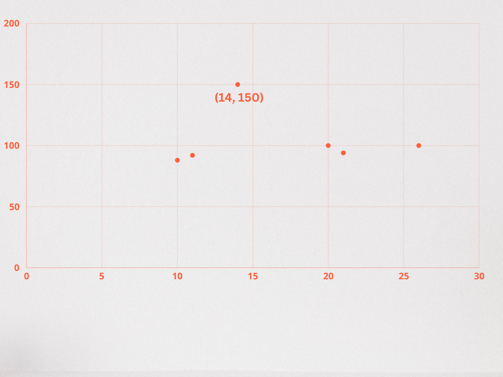
In the case of modern text embedding models, the number of dimensions is far greater, often 768, 1536, or more. The pgvector extension currently supports vectors of up to 2000 dimensions, with additional support recently added to store half vectors of up to 4000 dimensions. These high-dimensional vector representations allow for similarity search by comparing the values at each dimension of the vector.

Suppose we have a dataset of popular superheroes and access to a model that generates two-dimensional text embeddings for each description.

This is how we can use pgvector to store embeddings:

Create tables to store superheroes and their associated embeddings, using the vector data type. Here, we are specifying that our embeddings will have two dimensions in the description_embedding column.

CREATE TABLE superheroes (
  id int4 NULL,
  hero_name varchar(50) NULL,
  gender varchar(50) NULL,
  eye_color varchar(50) NULL,
  race varchar(50) NULL,
  hair_color varchar(50) NULL,
  height float4 NULL,
  publisher varchar(50) NULL,
  skin_color varchar(50) NULL,
  alignment varchar(50) NULL,
  weight float4 null,
  description text,
description_embedding vector(2),
);

Insert superheroes into the database.

INSERT INTO superheroes (superhero_name, superhero_description) VALUES 
('superman', 'possesses super strength, flight, and invulnerability, which he uses to fight for truth and justice on Earth'),
('batman', 'relies on his intellect, physical prowess, and an array of technological gadgets to combat crime and corruption'),
('the incredible hulk', 'transforms into a massive green creature with immense strength whenever he becomes angry');

Assign description_embeddings for each superhero description. Note: this is just an example. In a real-world scenario, a text embedding model would be used to generate a vector from the text stored in the description column.
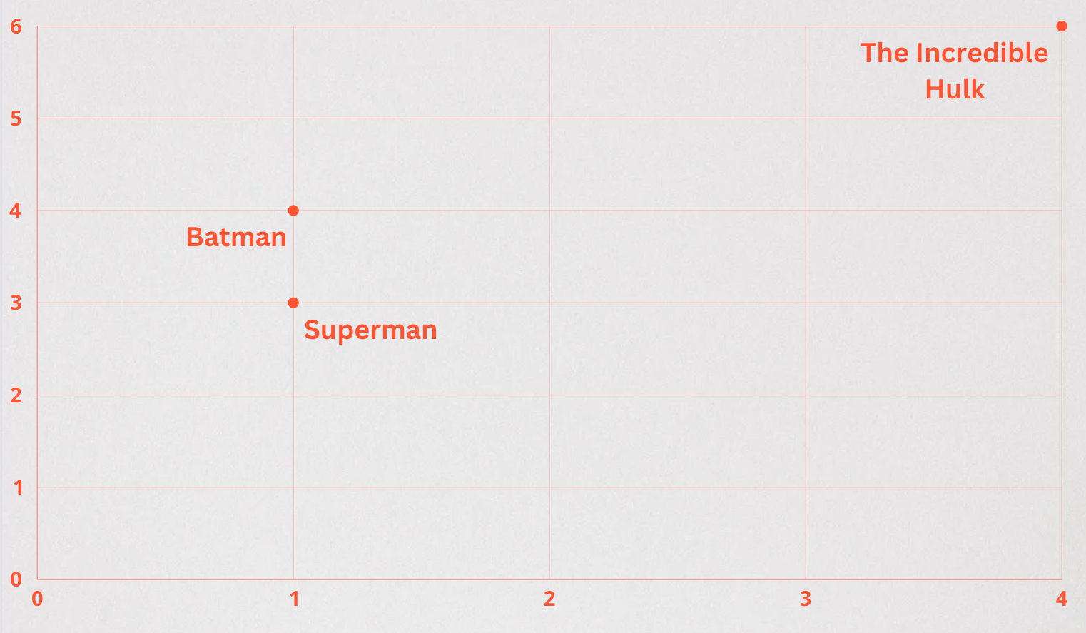
```
UPDATE superheroes 
SET description_embedding = '[1, 3]' 
WHERE id = 1; 

UPDATE superheroes 
SET description_embedding = '[1, 4]'
WHERE id = 2;

UPDATE superheroes 
SET description_embedding = '[4, 6]'
WHERE id = 3;
```

In this example, we’re able to plot the embeddings generated for each superhero description to visualize their likeness.

superhero description

In the next section we’ll cover how to query these embeddings using distance functions in pgvector.

Querying Embeddings

Pgvector allows us to query our records with the familiar PostgreSQL syntax. The most common way that vectors are queried is by distance.

There are several distance functions available in pgvector, with different practical applications.

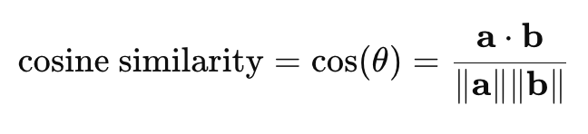
Cosine Distance (<=>): A measure of the cosine of the angle between two vectors. When doing an angular comparison, similarity is independent of vector magnitude. The smaller the cosine distance between vectors, the more similar they are. This function is often used in text comparison, when the orientation of vectors is more important than their magnitude.
The equation for cosine distance can be derived from cosine similarity:
- a⋅b: This is the dot product of the two vectors. It sums up the product of corresponding elements from the two vectors.
- ∥a∥: This denotes the magnitude (or norm) of vector a, calculated as
- ∥b∥: Similarly, this is the magnitude of vector b, calculated as
The range of cosine similarity is -1 to 1, with 1 indicating maximum similarity, 0 indicating no similarity, and -1 indicating maximum dissimilarity.
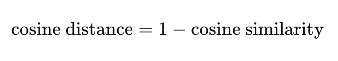
Here’s how cosine distance is derived from cosine similarity:
The range of cosine distance is 0 to 2, with 0 indicating no distance or maximum similarity, and 2 indicating maximum distance and thus maximum dissimilarity.
Here’s an example query using cosine distance with pgvector:
```
SELECT hero_name, description_embedding FROM superheroes ORDER BY description_embedding <=> ['1,5]' LIMIT 5;
 
 hero_name         | description_embedding 
Batman               [1,4]
Superman             [1,3]
The Incredible Hulk  [4,6]
```
While there isn’t a built-in function for querying directly by cosine similarity, this can be achieved algebraically. If Distance = 1 - Similarity, then Similarity = 1 - Distance.
Thus, we can order by cosine similarity:
```
SELECT 1 -  (description_embedding <=> '[3,1]') AS similarity FROM superheroes ORDER BY similarity;
```
Euclidean / L2 distance (<->): A measure of the straight line distance between two points. By comparing distances, it is assumed that a shorter distance represents more similarity.
```
SELECT * FROM superheroes ORDER BY description_embedding <-> '[3,1]';
```
Negative Inner Product (<#>): A measure of both the magnitude (distance) and direction (angle) between two vectors. Pgvector takes the inner product between two vectors and makes it negative, meaning a lower value indicates a greater similarity.
```
SELECT (description_embedding <#> '[3,1]') * -1 AS inner_product FROM superheroes;
...
```

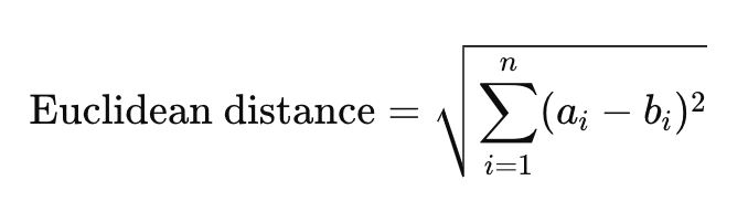
Let’s explore how we can pre-filter our data to increase the efficiency of our queries.

Pre-Filtering Data

Querying data using text embeddings is simple with the provided distance functions, but this can become a high latency operation over a large dataset. To improve the efficiency of our applications, pre-filter data in queries is a common strategy.

This is often seen in vector databases, where data is split into “chunks”. Each chunk has an associated metadata object, which allows the database to efficiently filter the data before executing a vector search.

This is a familiar practice for those using SQL databases. For instance, we might choose to pre-filter our superheroes by first limiting our dataset to Marvel superheroes.

SELECT COUNT(*) from superheroes;
 count 
-------
   734

SELECT COUNT(*) from superheroes where publisher = 'Marvel Comics';
 count 
-------
   388

We can reduce this further by searching for Marvel superheroes with blue eyes.

SELECT COUNT(*) from superheroes where publisher = 'Marvel Comics' AND eye_color = 'blue';
 count 
-------
   125

I’ve generated text embeddings for each character’s description, using a 1536-dimension OpenAI embedding model and stored this in the database using pgvector. By using the same model to generate embeddings for the text “has the power of invisibility,” we’re able to order by cosine distance.

SELECT hero_name from superheroes ORDER BY description_embedding <=> '[0.2452, 0.62356, ...] LIMIT 5';
    
hero_name    
-----------------
 Phantom
 Invisible Woman
 Vanisher
 Cloak
 Hollow
(5 rows)


Sort Method: top-N heapsort  Memory: 25kB
         ->  Seq Scan on superheroes  (cost=0.00..67.17 rows=734 width=18) (actual time=0.951..21.068 rows=734 loops=1)
Planning Time: 0.730 ms
Execution Time: 21.494 ms

Let’s execute the query on a reduced dataset by pre-filtering. In the following example, we’re searching for superheroes featured in DC Comics with blue eyes that have the power of invisibility.

First, we’ll create an index on the publisher column to improve the efficiency of our query.

CREATE INDEX publisher_idx on superheroes(publisher);

Now, we can execute the query and observe the query plan.

SELECT hero_name from superheroes where publisher = 'DC Comics' AND eye_color = 'blue' ORDER BY description_embedding <=> '[0.2452, 0.62356, ...] LIMIT 5';

hero_name
----------------
Rorschach
Misfit
Deadman
Scarecrow
John Constantine
(5 rows)

 Limit  (cost=68.27..68.28 rows=5 width=1095) (actual time=1.019..1.021 rows=5 loops=1)
   ->  Sort  (cost=68.27..68.43 rows=66 width=1095) (actual time=1.017..1.018 rows=5 loops=1)
         Sort Key: ((description_embedding <=> '[0.014116188,-0.00544635,...]'::vector)
         Sort Method: top-N heapsort  Memory: 33kB
         ->  Bitmap Heap Scan on superheroes  (cost=5.78..67.17 rows=66 width=1095) (actual time=0.075..0.936 rows=83 loops=1)
               Recheck Cond: ((publisher)::text = 'DC Comics'::text)
               Filter: ((eye_color)::text = 'blue'::text)
               Rows Removed by Filter: 132
               Heap Blocks: exact=57
               ->  Bitmap Index Scan on publisher_idx  (cost=0.00..5.76 rows=215 width=0) (actual time=0.032..0.032 rows=215 loops=1)
                     Index Cond: ((publisher)::text = 'DC Comics'::text)
 Planning Time: 0.146 ms
 Execution Time: 1.060 ms

Here, we’ve demonstrated that by creating an index and pre-filtering our dataset, latency has dropped significantly, from ~22ms to ~5ms.

Now, let’s examine how we can further improve query performance through the use of specialized vector indexes supported by pgvector.

Comparing Vector Indexes

By default, pgvector will execute an exact nearest neighbor query on the dataset by doing a full sequential scan of the data. As shown, this can result in slow queries when executed over a large dataset.

However, indexes are available to more efficiently query the data using approximate nearest neighbor (ANN) search. ANN algorithms allow us to sacrifice recall for the sake of speed, which is often a worthy tradeoff in our applications. Currently, pgvector supports the HSNW and IVFFlat indexes, and others are in development.

The prevailing index for most use cases is the Hierarchical Navigable Small Worlds (HSNW) index.

Hierarchical Navigable Small Worlds (HNSW)

A multi-layered graph-based index, HNSW is both performant and highly accurate.

As the name indicates, HNSW is an extension of Navigable Small Worlds, a graph-based algorithm for finding nearest neighbors. By making these graphs hierarchical, time and computational resources are reduced.

Below is a simplified representation of an HNSW traversal from entrypoint E to the ANN of a query vector, vertex 3:

HNSW traversal from entrypoint E to the ANN of a query vector, vertex 3

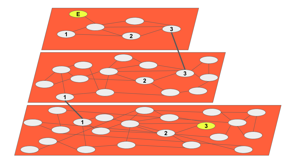
Each layer (graph) is more detailed than the one above it, allowing for high query performance by organizing vectors into “neighborhoods”. This is analogous to the experience of using digital maps, where zooming in increases the level of detail.

Insertions in HNSW indexes are iterative and indexing time increases as the data in the graph increases. This makes the index easy to manage, with an indexing time tradeoff.

CREATE INDEX superhero_description_hnsw_idx ON superheroes USING hnsw (description_embedding vector_cosine_ops) WITH (m = 4, ef_construction = 10);

Limit  (cost=100.18..101.82 rows=5 width=1095) (actual time=0.849..0.912 rows=5 loops=1)
   ->  Index Scan using superheroes_description_hnsw_idx on superheroes  (cost=100.18..341.35 rows=734 width=1095) (actual time=0.846..0.909 rows=5 loops=1)
         Order By: (description_embedding <=> '[0.014116188,-0.00544635,...]'::vector)
 Planning Time: 0.185 ms
 Execution Time: 0.649 ms

Inverted File Flat (IVFFlat)

The IVFFlat index differs from HNSW, in that it clusters data into lists at build time. By doing so a search vector can be compared to the centroid of each cluster (also know as a list) to determine which is most closely related.

Inverted File Flat

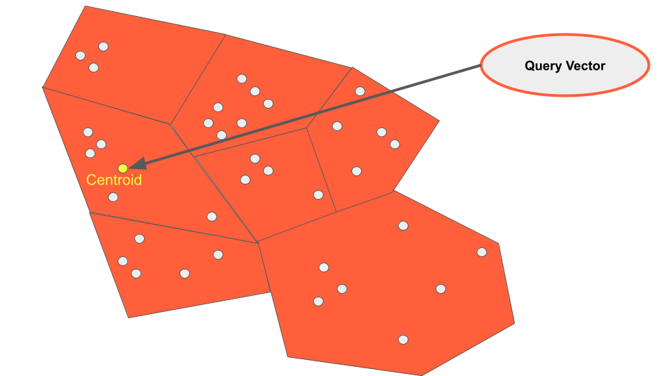
By configuring how many lists we wish to visit during a query, we can adjust the tradeoff between recall and speed. This is better known as setting the number of “probes”. By setting more probes on our queries more lists will be searched, yielding better results.

For instance, if you’d like to visit 10 lists to improve recall in our queries, you can set the following parameter:

SET ivfflat.probes = 10;

Similarly, the number of lists can be set, with a greater number of lists resulting in less vectors per list. This will improve the speed of queries by reducing the number of vectors in the search space, but could lead to recall errors by excluding valid data points.

Lists can be set on the index at creation time. For instance, the following segments data into 50 lists:

CREATE INDEX superhero_description_ivfflat_idx ON superheroes USING ivfflat (description_embedding vector_cosine_ops) WITH (lists = 50);


SELECT hero_name FROM superheroes ORDER BY description_embedding <=> '[0.014116188,-0.00544635,... ]' LIMIT 5;

Limit  (cost=40.11..40.51 rows=5 width=18) (actual time=0.477..0.538 rows=5 loops=1)
  ->  Index Scan using superhero_description_ivfflat_idx on superheroes  (cost=40.11..98.10 rows=734 width=18) (actual time=0.476..0.535 rows=5 loops=1)
        Order By: (description_embedding <=> '[0.014116188,-0.00544635,...]'::vector)
Planning Time: 0.142 ms
Execution Time: 0.567 ms

Comparison

Let’s compare the two indexes at a glance:

Index	Build Speed	Query Speed	Requires Rebuild on Updates
HNSW	Slowest	Fast	No
IVFFlat	Fastest	Slowest	Yes

HNSW

Graph based
Organizes vectors into neighborhoods
Iterative insertions
Insertion time increases as data in the graph increases

When to use:

Frequent data changes
High query performance and recall

IVFFlat

K-means based
Organizes vectors into lists
Requires pre-populated data
Insertion time bounded by number of lists

When to use:

Data is mostly static
Fast indexing

Scaling with YugabyteDB

Let’s explore how we can leverage distributed SQL to make our applications even more scalable and resilient.

Here are some key reasons that AI applications using pgvector benefit from distributed PostgreSQL databases, like YugabyteDB:

Embeddings consume a lot of storage and memory. For instance, an OpenAI model with 1536 dimensions takes up ~57GB of space for 10 million records. Scaling horizontally provides the space required to store vectors.
Vector similarity search is very compute-intensive. By scaling out to multiple nodes, applications have access to unbound CPU and GPU limits.
Service interruptions won’t be an issue. The database will be resilient to node, data center or regional outages, meaning AI applications will never experience downtime as a result of the database tier.

YugabyteDB is a distributed SQL database built on PostgreSQL. Feature and runtime compatible with Postgres, it allows you to reuse the libraries, drivers, tools and frameworks created for the standard version of Postgres.

YugabyteDB has pgvector compatibility and provides all of the functionality found in native PostgreSQL. This makes it ideal for those looking to level-up their AI applications.

Here’s how you can run a 3-node YugabyteDB cluster locally in Docker.

Create a directory to store data locally.
```
mkdir ~/yb_docker_data
```
Create a Docker network
```
docker network create custom-network
```

Deploy a 3-node cluster to this network.

docker run -d --name yugabytedb-node1 --net custom-network \
      -p 15433:15433 -p 7001:7000 -p 9001:9000 -p 5433:5433 \
      -v ~/yb_docker_data/node1:/home/yugabyte/yb_data --restart unless-stopped \
      yugabytedb/yugabyte:latest \
      bin/yugabyted start \
      --base_dir=/home/yugabyte/yb_data --background=false

docker run -d --name yugabytedb-node2 --net custom-network \
      -p 15434:15433 -p 7002:7000 -p 9002:9000 -p 5434:5433 \
      -v ~/yb_docker_data/node2:/home/yugabyte/yb_data --restart unless-stopped \
      yugabytedb/yugabyte:latest \
      bin/yugabyted start --join=yugabytedb-node1 \
      --base_dir=/home/yugabyte/yb_data --background=false

docker run -d --name yugabytedb-node3 --net custom-network \
      -p 15435:15433 -p 7003:7000 -p 9003:9000 -p 5435:5433 \
      -v ~/yb_docker_data/node3:/home/yugabyte/yb_data --restart unless-stopped \
      yugabytedb/yugabyte:latest \
      bin/yugabyted start --join=yugabytedb-node1 \
      --base_dir=/home/yugabyte/yb_data --background=false

Conclusion

The pgvector extension is yet another example of the open source community adding functionality to PostgreSQL, making it an ideal database choice for modern applications.

With additional distance functions, indexes, and more in development, pgvector is continuing to add value to those adding AI functionality to their applications. Developers seeking to add resilience and scalability to their AI applications can turn to YugabyteDB, to distribute their data horizontally without sacrificing performance.

Interested in learning more about building generative AI applications with YugabyteDB? Check out these resources:

June 20, 2024